GIS I Lab IV: Custom Project

INTRODUCTION

The following lab gave the freedom to explore GIS applications and solve a spatial question. The goal was to obtain data from multiple sources, use a variety of GIS tools, and use statistics to provide a solution. Additionally, an effort was made to solve a unique spatial question to showcase the extent to which GIS can be applied. Specifically, the objective was to find the location in which the best odds at finding a potential girlfriend based on personal criteria exists.

This included all women aged 20-24 who live 20 miles away from the nearest city. Basically put, rural land was located and US Census data for that county was used to calculate how many women should be expected to live in that region.  Finally, a town was selected in the region with the best odds. 

METHODOLOGY

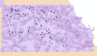
First, US rivers and streams, and US cities data was obtained and clipped within the state of Wisconsin. Next, a buffer of 50 miles was executed around Wisconsin cities followed by a dissolve function to form a single shapefile. This shapefile was then erased by all county land to form a shapefile of country land in Wisconsin. This was then intersected by county boundaries to form separate shapes divided among counties.

US Census data was obtained containing Wisconsin county area, the number of men and women, and age subdivisions within each county. First, the number of women was divided from the number of men to calculate the percent of women for each county. Next, the percent of women was multiplied by the age group of 20-24 to give an estimated number of females within the county. Finally, the estimated number of females was divided by the total area of the county to give the number of acres per female.

The shapefile of country areas was then spatially joined with the data from the US Census data calculations. A final calculation was made dividing the county area by the number of acres per female resulting in an estimated number of females per country area in that county.

All areas were then mapped using a rounded natural breaks method with five classes. The country areas containing the most estimated females were then overlaid by the Wisconsin rivers and streams to determine whether they were in near proximity to a stream. Finally, a town was selected that most fittingly matched all criteria.

For a visual representation of all input layers, functions performed, and output layers, Figure 1 shows the process of tasks performed. 

RESULTS

From the criteria of 20-24-year-old-women who live 50 miles away from any city, Figure 2 represents the estimated number per country area in each county. Marinette, Douglas, and Oneida are the top-tier with 33, 26, and 21, respectively and can be seen as the darkest shade of pink on Figure 3.  

Of the top-tier of estimated women based on criteria, the Marinette country area sits along five rivers and streams, whereas Douglass possesses two, and Oneida with none as shown by Figure 3. Based on access to rivers and streams, the Marinette country location is the clear favorite.

 From both the number of females estimated in country areas per county and access to rivers and streams, the Marinette location is the prime location. Within this area rests the town of Silver Creek, which has access to three streams. In fact, it’s the only town listed in Google maps in any of the top-tier country zones of the Marinette, Douglass, or Oneida counties.

CONCLUSION

Based on results gathered, a prime location was generated as the town of Silver Cliff located in Marinette County, Wisconsin. It provides the best odds at locating a girlfriend 20-24 years old that lives 50 miles away from a city and has access to a river or stream. This would be helpful to college-aged single men who have interests in hunting and fishing.

Although this is a pretty absurd use for GIS, this lab showcases the very real extent to which GIS can be used. Statistics from the US Census Bureau, shapefiles from the DNR, and additional data from ESRI can be combined to find solutions and inform important decisions. There is a plethora of data available that, with skills in data analysis and GIS functions, allows to find customized solutions. The results of any GIS project gives a spatial understanding, supports it with statistics and data, and is used to inform decisions. In this case, it looks as though one should move to Silver Creek if in search of a country soulmate.

Another important lesson to be gained from this lab was using data responsibly. If this lab wasn’t interpreted with humor, it could easily be viewed as an irresponsible use of data. Using US Census Data on women for personal use would be irresponsible. For this lab’s purpose, it was instead intended to showcase the aforementioned qualities of GIS and to be intentionally humorous. 

SOURCES

US cities and rivers and streams data obtained from the ESRI database.

WI state and county boundaries obtained from the Wisconsin Department of Natural Resources.

Wisconsin county population data obtained from the US Census Bureau.

GIS I Lab III: Vector Analysis with ArcGIS

INTRODUCTION

This lab demonstrates the ability to use various geoprocessing tools for vector analysis in arcGIS and a basic introduction to ArcGIS Python. Using a GPS MS Excel file of black bear locations in central Marquette County, Michigan, criteria was chosen to build a data flow model by using python script to find suitable bear habitat in the study area. This information was then used to recommend territory suitable for bears and away from urban environments to the DNR. 

For the area of interest (AOI) of central Marquetty County, Michigan, the political boundaries of state, county, and DNR management were stored under a feature class and the study area, streams, and land cover were stored under another feature class while bear locations were stores as simple x,y coordinates all under a single geodatabase.

METHODOLOGY

First, the x,y coordinates of bear locations were converted into an event theme, which gives the layer a spatial quality with limitations. The layer was then exported as a feature class under the geodatabase to begin functions.

Land Cover & Proximity to Streams

In order to discover bear habitat, a spatial join combined bear locations with land cover. A summary of this new spatial join layer gave the most common land cover types bears were found. The top three land cover zones were chosen and made into a separate layer.

In order to further delineate bear territory, a buffer of 500 meters was created around streams. The bear locations was then spatially joined with this stream layer to discover the number of bears within 500 meters of a stream.

Creating a Bear Habitat Zone

Based on results from land cover and proximity to streams, a bear habitat was created using an intersect function of these two layers. To aggregate the output layer into a single land area, the dissolve function was used based on the stream buffer field.

DNR Bear Habitat Land

After aggregating all DNR land, a series of clips were performed to only show DNR land that contained bear habitat according to the previous results.

DNR Bear Habitat Away from Urban Environment

A separate layer was created from land cover based on urban and built up land. A 5 kilometer buffer was then created around this layer. Finally using the erase function, all DNR bear habitat land was erased within the 5 km buffer zone.

Python Script

After all analysis was completed, python script commands were performed to create a buffer around streams and intersect with bear habitat lands. Figure 1 shows the python script performed and the results gathered into a personal geodatabase.

RESULTS

The AOI in central Marquetty County, Michigan after adding all feature classes from the dataset is shown in Figure 2.

Land Cover

After combining bear locations with areas of land cover, a summary statistics of the output layer was performed to give the most common land covers bears were located as shown by Figure 3. According to the results, mixed forest land, forested wetlands, and evergreen forest land were first, second, and third, respectively. 

From these three land cover areas which hold the majority of bears, a new layer was created.

Proximity to Streams

Figure 4 shows the dark purple zones as a 500 meter buffer from every stream in the AOI. After a spatial join of the buffer area with bear locations was performed, an output of bear locations within 500 meters of a stream is visible by the blue points. 

Out of the 68 bear locations, 49 of the bears were located within this buffer zone. According to biologists, if the percentage would exceed 30%, the data would be important. Therefore, at a 72% rate, this data would be considered highly significant.

Creating a Bear Habitat Zone

An intersection between the layer that held the top three land cover areas likely to contain bears and the buffer of 500 meters from a stream or river was produced as indicated by Figure 5. This intersection was based off the 500-meter buffer and therefore, the output drew from multiple polygons creating a dis-contiguous zone. 

This zone was aggregated into a single, cohesive layer using the dissolve tool as indicated by the tan area in Figure 6. 

DNR Bear Habitat Land

After dissolving all DNR land into a single unit, and a series of clips later, Figure 7 shows all DNR land in the AOI that are suitable for bears. 

DNR Bear Habitat Away from Urban Environment

In Figure 8, the urban and built up lands are indicated by the gray territory, while the green lands represent DNR bear habitat land within a 5 km buffer zone of urban environment. Finally, the red areas represent all DNR bear habitat land located away from the urban environment. 

Overview of Tasks Performed

Figure 9 shows the input and output layers used and the functions performed using ArcGIS including spatial joins, summaries, queries, buffers, clips, dissolves, and erases to achieve a final product. 

Figure 10 is the completed project, accurately showing all bear habitat, urban areas, streams, DNR bear habitat lands 5km away from urban areas, GPS locations of bears, and a reference map showing the location of the area of study. 

To find this data, the tasks performed and knowledge gained was both valuable and enjoyable. With a comprehensive knowledge of the tools in ArcGIS, there are various strategies available to derive a final product. The outlines of a project, such as DNR recommendations of suitable bear habitat, allow for creativity and full use of GIS functions. 

SOURCES

All of the data were downloaded from the State of Michigan Open GIS Data http://gis.michigan.opendata.arcgis.com/
Landcover obtained from USGS NLCD
http://www.mcgi.state.mi.us/mgdl/nlcd/metadata/nlcdshp.html
DNR management units
http://www.dnr.state.mi.us/spatialdatalibrary/metadata/wildlife_mgmt_units.htm
Streams from
http://www.mcgi.state.mi.us/mgdl/framework/metadata/Marquette.html